Take-home Exercise 3: Predicting HDB Public Housing Resale Pricies using Geographically Weighted Methods

1 Setting The Scene

Housing is an essential component of household wealth worldwide. Buying a housing has always been a major investment for most people. The price of housing is affected by many factors. Some of them are global in nature such as the general economy of a country or inflation rate. Others can be more specific to the properties themselves. These factors can be further divided to structural and locational factors. Structural factors are variables related to the property themselves such as the size, fitting, and tenure of the property. Locational factors are variables related to the neighbourhood of the properties such as proximity to childcare centre, public transport service and shopping centre.

Conventional, housing resale prices predictive models were built by using Ordinary Least Square (OLS) method. However, this method failed to take into consideration that spatial autocorrelation and spatial heterogeneity exist in geographic data sets such as housing transactions. With the existence of spatial autocorrelation, the OLS estimation of predictive housing resale pricing models could lead to biased, inconsistent, or inefficient results (Anselin 1998). In view of this limitation, Geographical Weighted Models were introduced for calibrating predictive model for housing resale prices.

2 The Task

In this take-home exercise, we are tasked to predict HDB resale prices at the sub-market level (i.e. HDB 3-room, HDB 4-room and HDB 5-room) for the month of January and February 2023 in Singapore. The predictive models must be built by using by using conventional OLS method and GWR methods. You are also required to compare the performance of the conventional OLS method versus the geographical weighted methods.

3 Installing Packages

  • sf: used for importing, managing and processing geospatial data

  • tidyverse: collection of R packages designed for data wrangling

  • tmap: used for creating thematic maps, such as chloropleth and bubble maps

  • httr: used to make API calls, such as GET requests

  • jsonlite: a JSON parser that can convert from JSON to the appropraite R data types

  • rvest: Wrappers around the ‘xml2’ and ‘httr’ packages to make it easy to download, then manipulate, HTML and XML.

  • sp: Classes and methods for spatial data

  • ggpubr: used for multivariate data visualisation & analysis

  • corrplot: used for multivariate data visualisation & analysis

  • broom: The broom package takes the messy output of built-in functions in R, such as lm, nls, or t.test, and turns them into tidy tibbles.

  • olsrr: used for building least squares regression models

  • spdep: used to create spatial weights matrix objects, global and local spatial autocorrelation statistics and related calculations (e.g. spatially lag attributes)

  • GWmodel: provides a collection of localised spatial statistical methods, such as summary statistics, principal components analysis, discriminant analysis and various forms of GW regression

  • devtools: used for installing any R packages which is not available in RCRAN

  • lwgeom: Functions for SF

  • maptools: Tools for handling spatial objects

  • matrixstats: a set of high-performing functions for operating on rows and columns of matrices

  • units: Measurement Units for R Vectors

  • metrics: Evaluation metrics for machine learning

  • gtsummary: provides an elegant and flexible way to create publication-ready analytical and summary tables using the R programming language

  • rsample: The rsample package provides functions to create different types of resamples and corresponding classes for their analysis

  • spatialml: allows for a geographically weighted random forest regression to include a function to find the optimal bandwidth

packages <- c('sf', 'tidyverse', 'tmap', 'httr', 'jsonlite', 'rvest', 
              'sp', 'ggpubr', 'corrplot', 'broom',  'olsrr', 'spdep', 
              'GWmodel', 'devtools', 'lwgeom', 'maptools', 'matrixStats', 'units', 'Metrics', 'gtsummary', 'rsample', 'SpatialML')

for(p in packages){
  if(!require(p, character.only = T)){
    install.packages(p, repos = "http://cran.us.r-project.org")
  }
  library(p, character.only = T)
}
Loading required package: sf
Linking to GEOS 3.9.3, GDAL 3.5.2, PROJ 8.2.1; sf_use_s2() is TRUE
Loading required package: tidyverse
── Attaching packages ─────────────────────────────────────── tidyverse 1.3.2 ──
✔ ggplot2 3.4.1      ✔ purrr   1.0.1 
✔ tibble  3.1.8      ✔ dplyr   1.0.10
✔ tidyr   1.3.0      ✔ stringr 1.5.0 
✔ readr   2.1.3      ✔ forcats 0.5.2 
── Conflicts ────────────────────────────────────────── tidyverse_conflicts() ──
✖ dplyr::filter() masks stats::filter()
✖ dplyr::lag()    masks stats::lag()
Loading required package: tmap

Loading required package: httr

Loading required package: jsonlite


Attaching package: 'jsonlite'


The following object is masked from 'package:purrr':

    flatten


Loading required package: rvest


Attaching package: 'rvest'


The following object is masked from 'package:readr':

    guess_encoding


Loading required package: sp

Loading required package: ggpubr

Loading required package: corrplot

corrplot 0.92 loaded

Loading required package: broom

Loading required package: olsrr


Attaching package: 'olsrr'


The following object is masked from 'package:datasets':

    rivers


Loading required package: spdep

Loading required package: spData

To access larger datasets in this package, install the spDataLarge
package with: `install.packages('spDataLarge',
repos='https://nowosad.github.io/drat/', type='source')`

Loading required package: GWmodel

Loading required package: maptools

Checking rgeos availability: TRUE
Please note that 'maptools' will be retired during 2023,
plan transition at your earliest convenience;
some functionality will be moved to 'sp'.

Loading required package: robustbase

Loading required package: Rcpp

Loading required package: spatialreg

Loading required package: Matrix


Attaching package: 'Matrix'


The following objects are masked from 'package:tidyr':

    expand, pack, unpack


Attaching package: 'spatialreg'


The following objects are masked from 'package:spdep':

    get.ClusterOption, get.coresOption, get.mcOption,
    get.VerboseOption, get.ZeroPolicyOption, set.ClusterOption,
    set.coresOption, set.mcOption, set.VerboseOption,
    set.ZeroPolicyOption


Welcome to GWmodel version 2.2-9.

Loading required package: devtools

Loading required package: usethis

Loading required package: lwgeom

Linking to liblwgeom 3.0.0beta1 r16016, GEOS 3.9.1, PROJ 7.2.1
Warning in fun(libname, pkgname): GEOS versions differ: lwgeom has 3.9.1 sf has
3.9.3
Warning in fun(libname, pkgname): PROJ versions differ: lwgeom has 7.2.1 sf has
8.2.1
Loading required package: matrixStats

Attaching package: 'matrixStats'

The following objects are masked from 'package:robustbase':

    colMedians, rowMedians

The following object is masked from 'package:dplyr':

    count

Loading required package: units
udunits database from C:/R-4.2.2/library/units/share/udunits/udunits2.xml
Loading required package: Metrics
Loading required package: gtsummary
Loading required package: rsample

Attaching package: 'rsample'

The following object is masked from 'package:Rcpp':

    populate

Loading required package: SpatialML
Loading required package: ranger
Loading required package: caret
Loading required package: lattice

Attaching package: 'caret'

The following objects are masked from 'package:Metrics':

    precision, recall

The following object is masked from 'package:httr':

    progress

The following object is masked from 'package:purrr':

    lift

4 The Data

The following datasets are derived from the respective sources.

library(knitr)
library(kableExtra)
Warning: package 'kableExtra' was built under R version 4.2.3

Attaching package: 'kableExtra'
The following object is masked from 'package:dplyr':

    group_rows
# Create a table with 3 columns
table <- data.frame(
  Type = c("Aspatial", "Geospatial", "Geospatial", "Geospatial", "Geospatial", "Geospatial", "Geospatial", "Geospatial", "Geospatial", "Geospatial", "Geospatial"),
  Dataset = c("HDB Resale Data", "2019 Subzone Boundary", "Mrt Station", "Bus Stop", "Shopping Mall", "Parks and Nature Reserve", "Kindergarten", "Hawker Centre", "Childare Centre", "Eldercare", "Supermarket"),
  Source = c("[Data.gov.sg](https://data.gov.sg/dataset/resale-flat-prices)", 'Prof.Kam', "[datamall.lta.gov.sg](https://datamall.lta.gov.sg/content/datamall/en/static-data.html)", "[datamall.lta.gov.sg](https://datamall.lta.gov.sg/content/datamall/en/static-data.html)", "[Github](https://github.com/ValaryLim/Mall-Coordinates-Web-Scraper)", "[Onemap.gov.sg](https://www.onemap.gov.sg/main/v2/essentialamenities)", "[Onemap.gov.sg](https://www.onemap.gov.sg/main/v2/themes)", "[Onemap.gov.sg](https://www.onemap.gov.sg/main/v2/themes)", "[Onemap.gov.sg](https://www.onemap.gov.sg/main/v2/themes)", "[Onemap.gov.sg](https://data.gov.sg/dataset/eldercare-services)", "[Onemap.gov.sg](https://data.gov.sg/dataset/supermarkets)")
                )

# Format the table using kable
kable(table, caption = "Datasets", align = "c") %>%
  kable_styling(bootstrap_options = "striped", full_width = F)
Datasets
Type Dataset Source
Aspatial HDB Resale Data [Data.gov.sg](https://data.gov.sg/dataset/resale-flat-prices)
Geospatial 2019 Subzone Boundary Prof.Kam
Geospatial Mrt Station [datamall.lta.gov.sg](https://datamall.lta.gov.sg/content/datamall/en/static-data.html)
Geospatial Bus Stop [datamall.lta.gov.sg](https://datamall.lta.gov.sg/content/datamall/en/static-data.html)
Geospatial Shopping Mall [Github](https://github.com/ValaryLim/Mall-Coordinates-Web-Scraper)
Geospatial Parks and Nature Reserve [Onemap.gov.sg](https://www.onemap.gov.sg/main/v2/essentialamenities)
Geospatial Kindergarten [Onemap.gov.sg](https://www.onemap.gov.sg/main/v2/themes)
Geospatial Hawker Centre [Onemap.gov.sg](https://www.onemap.gov.sg/main/v2/themes)
Geospatial Childare Centre [Onemap.gov.sg](https://www.onemap.gov.sg/main/v2/themes)
Geospatial Eldercare [Onemap.gov.sg](https://data.gov.sg/dataset/eldercare-services)
Geospatial Supermarket [Onemap.gov.sg](https://data.gov.sg/dataset/supermarkets)

4.1 Importing Aspatial Data

hdb_resale <- read_csv("data/aspatial/resale-flat-prices-based-on-registration-date-from-jan-2017-onwards.csv")
Rows: 148479 Columns: 11
── Column specification ────────────────────────────────────────────────────────
Delimiter: ","
chr (8): month, town, flat_type, block, street_name, storey_range, flat_mode...
dbl (3): floor_area_sqm, lease_commence_date, resale_price

ℹ Use `spec()` to retrieve the full column specification for this data.
ℹ Specify the column types or set `show_col_types = FALSE` to quiet this message.

Let’s see what aspatial data we are working with

head(hdb_resale)
# A tibble: 6 × 11
  month   town     flat_…¹ block stree…² store…³ floor…⁴ flat_…⁵ lease…⁶ remai…⁷
  <chr>   <chr>    <chr>   <chr> <chr>   <chr>     <dbl> <chr>     <dbl> <chr>  
1 2017-01 ANG MO … 2 ROOM  406   ANG MO… 10 TO …      44 Improv…    1979 61 yea…
2 2017-01 ANG MO … 3 ROOM  108   ANG MO… 01 TO …      67 New Ge…    1978 60 yea…
3 2017-01 ANG MO … 3 ROOM  602   ANG MO… 01 TO …      67 New Ge…    1980 62 yea…
4 2017-01 ANG MO … 3 ROOM  465   ANG MO… 04 TO …      68 New Ge…    1980 62 yea…
5 2017-01 ANG MO … 3 ROOM  601   ANG MO… 01 TO …      67 New Ge…    1980 62 yea…
6 2017-01 ANG MO … 3 ROOM  150   ANG MO… 01 TO …      68 New Ge…    1981 63 yea…
# … with 1 more variable: resale_price <dbl>, and abbreviated variable names
#   ¹​flat_type, ²​street_name, ³​storey_range, ⁴​floor_area_sqm, ⁵​flat_model,
#   ⁶​lease_commence_date, ⁷​remaining_lease

4.1.1 Filtering HDB Resale Aspatial Data

From the results above in section 3.1, we can see that the data starts from Year 2017. But for this assignment we are only focusing on 1st January 2021 to 31st December 2022. Thus the below code chunk will do the filtering.

hdb_filtered_resale <- filter(hdb_resale, flat_type == "4 ROOM") %>%
  filter(month >= "2021-01" & month <= "2023-02")

Now let us see what data we are working with and see if the data is what we have filtered.

head(hdb_filtered_resale)
# A tibble: 6 × 11
  month   town     flat_…¹ block stree…² store…³ floor…⁴ flat_…⁵ lease…⁶ remai…⁷
  <chr>   <chr>    <chr>   <chr> <chr>   <chr>     <dbl> <chr>     <dbl> <chr>  
1 2021-01 ANG MO … 4 ROOM  547   ANG MO… 04 TO …      92 New Ge…    1981 59 yea…
2 2021-01 ANG MO … 4 ROOM  414   ANG MO… 01 TO …      92 New Ge…    1979 57 yea…
3 2021-01 ANG MO … 4 ROOM  509   ANG MO… 01 TO …      91 New Ge…    1980 58 yea…
4 2021-01 ANG MO … 4 ROOM  467   ANG MO… 07 TO …      92 New Ge…    1979 57 yea…
5 2021-01 ANG MO … 4 ROOM  571   ANG MO… 07 TO …      92 New Ge…    1979 57 yea…
6 2021-01 ANG MO … 4 ROOM  134   ANG MO… 07 TO …      98 New Ge…    1978 56 yea…
# … with 1 more variable: resale_price <dbl>, and abbreviated variable names
#   ¹​flat_type, ²​street_name, ³​storey_range, ⁴​floor_area_sqm, ⁵​flat_model,
#   ⁶​lease_commence_date, ⁷​remaining_lease

From the above output, it looks like it is according to the specifications that we wanted now.

The below code chunks will check if the months, room type are what we want to work with.

4.1.2 Checking for 4 Room Type Period

unique(hdb_filtered_resale$flat_type)
[1] "4 ROOM"

From the above output, the “hdb_resale_filtered” only consists of 4 Room which reflects our filter code in 3.1.1.

4.1.3 Checking for unique months

unique(hdb_filtered_resale$month)
 [1] "2021-01" "2021-02" "2021-03" "2021-04" "2021-05" "2021-06" "2021-07"
 [8] "2021-08" "2021-09" "2021-10" "2021-11" "2021-12" "2022-01" "2022-02"
[15] "2022-03" "2022-04" "2022-05" "2022-06" "2022-07" "2022-08" "2022-09"
[22] "2022-10" "2022-11" "2022-12" "2023-01" "2023-02"

From the above output, the month and year ranges from January 2021 to December 2022 which is what we want.

4.2 Importing Geospatial Data

4.2.1 2019 SG Subzone Boundary

mpsz <- st_read(dsn = "data/geospatial", layer = "MPSZ-2019")
Reading layer `MPSZ-2019' from data source 
  `C:\HoYongQuan\IS415-GAA(New)\Take-home_Ex\Take-home_Ex03\data\geospatial' 
  using driver `ESRI Shapefile'
Simple feature collection with 332 features and 6 fields
Geometry type: MULTIPOLYGON
Dimension:     XY
Bounding box:  xmin: 103.6057 ymin: 1.158699 xmax: 104.0885 ymax: 1.470775
Geodetic CRS:  WGS 84

4.2.2 Bus Stops

bus_stop_sf <- st_read(dsn = "data/geospatial", layer = "BusStop")
Reading layer `BusStop' from data source 
  `C:\HoYongQuan\IS415-GAA(New)\Take-home_Ex\Take-home_Ex03\data\geospatial' 
  using driver `ESRI Shapefile'
Simple feature collection with 5159 features and 3 fields
Geometry type: POINT
Dimension:     XY
Bounding box:  xmin: 3970.122 ymin: 26482.1 xmax: 48284.56 ymax: 52983.82
Projected CRS: SVY21

4.2.3 Mrt Stations

mrt <- read.csv("data/geospatial/mrtsg.csv")

4.2.3.1 Converting MRT Station dataframe file to SF

mrt_sf <- st_as_sf(mrt, coords = c("Longitude", "Latitude"), crs = 4326)

4.2.4 Elderly Care

elderly_care_sf <- st_read(dsn = "data/geospatial", layer = "ELDERCARE")
Reading layer `ELDERCARE' from data source 
  `C:\HoYongQuan\IS415-GAA(New)\Take-home_Ex\Take-home_Ex03\data\geospatial' 
  using driver `ESRI Shapefile'
Simple feature collection with 133 features and 18 fields
Geometry type: POINT
Dimension:     XY
Bounding box:  xmin: 14481.92 ymin: 28218.43 xmax: 41665.14 ymax: 46804.9
Projected CRS: SVY21

4.2.5 Childcare Center

childcare_sf <- st_read(dsn = "data/geospatial", layer = "CHILDCARE")
Reading layer `CHILDCARE' from data source 
  `C:\HoYongQuan\IS415-GAA(New)\Take-home_Ex\Take-home_Ex03\data\geospatial' 
  using driver `ESRI Shapefile'
Simple feature collection with 1545 features and 15 fields
Geometry type: POINT
Dimension:     XY
Bounding box:  xmin: 11203.01 ymin: 25667.6 xmax: 45404.24 ymax: 49300.88
Projected CRS: WGS_1984_Transverse_Mercator

4.2.6 Kindergarten

kindergarten_sf <- st_read(dsn = "data/geospatial", layer = "KINDERGARTENS")
Reading layer `KINDERGARTENS' from data source 
  `C:\HoYongQuan\IS415-GAA(New)\Take-home_Ex\Take-home_Ex03\data\geospatial' 
  using driver `ESRI Shapefile'
Simple feature collection with 448 features and 15 fields
Geometry type: POINT
Dimension:     XY
Bounding box:  xmin: 11909.7 ymin: 25596.33 xmax: 43395.47 ymax: 48562.06
Projected CRS: SVY21

4.2.7 Hawker Centre

hawker_centre_sf <- st_read(dsn = "data/geospatial", layer = "HAWKERCENTRE")
Reading layer `HAWKERCENTRE' from data source 
  `C:\HoYongQuan\IS415-GAA(New)\Take-home_Ex\Take-home_Ex03\data\geospatial' 
  using driver `ESRI Shapefile'
Simple feature collection with 125 features and 21 fields
Geometry type: POINT
Dimension:     XY
Bounding box:  xmin: 12874.19 ymin: 28355.97 xmax: 45241.4 ymax: 47872.53
Projected CRS: SVY21

4.2.8 Supermarket

supermarket_sf <- st_read(dsn = "data/geospatial", layer = "SUPERMARKETS")
Reading layer `SUPERMARKETS' from data source 
  `C:\HoYongQuan\IS415-GAA(New)\Take-home_Ex\Take-home_Ex03\data\geospatial' 
  using driver `ESRI Shapefile'
Simple feature collection with 526 features and 8 fields
Geometry type: POINT
Dimension:     XY
Bounding box:  xmin: 4901.188 ymin: 25529.08 xmax: 46948.22 ymax: 49233.6
Projected CRS: SVY21

4.2.9 Parks and Nature Parks

parks_sf <- st_read(dsn = "data/geospatial", layer = "NATIONALPARKS")
Reading layer `NATIONALPARKS' from data source 
  `C:\HoYongQuan\IS415-GAA(New)\Take-home_Ex\Take-home_Ex03\data\geospatial' 
  using driver `ESRI Shapefile'
Simple feature collection with 352 features and 15 fields
Geometry type: POINT
Dimension:     XY
Bounding box:  xmin: 12373.11 ymin: 21869.93 xmax: 46735.95 ymax: 49231.09
Projected CRS: SVY21

4.2.10 Marking CBD coordinates

name <- c('CBD')
latitude = c(1.287953)
longitude = c(103.851784)
cbd <- data.frame(name, latitude, longitude)

4.2.10.1 Converting CBD data.frame to sf

cbd_sf <- st_as_sf(cbd, coords = c("longitude", "latitude"), crs = 4326)

4.2.11 Shopping Malls

shopping_mall <- read.csv("data/geospatial/mall_coordinates.csv")

4.2.11.1 Converting Shopping Mall Data Frame to SF

shopping_mall_sf <- st_as_sf(shopping_mall,coords = c("longitude", "latitude"),crs = 4326)

4.2.12 Checking for Invalid Geometries for the above imported Geospatial data

length(which(st_is_valid(mpsz) == FALSE))
[1] 6
length(which(st_is_valid(bus_stop_sf) == FALSE))
[1] 0
length(which(st_is_valid(mrt_sf) == FALSE))
[1] 0
length(which(st_is_valid(elderly_care_sf) == FALSE))
[1] 0
length(which(st_is_valid(childcare_sf) == FALSE))
[1] 0
length(which(st_is_valid(kindergarten_sf) == FALSE))
[1] 0
length(which(st_is_valid(hawker_centre_sf) == FALSE))
[1] 0
length(which(st_is_valid(supermarket_sf) == FALSE))
[1] 0
length(which(st_is_valid(parks_sf) == FALSE))
[1] 0
length(which(st_is_valid(cbd_sf) == FALSE))
[1] 0
length(which(st_is_valid(shopping_mall_sf) == FALSE))
[1] 0

From the above output, we can see that there are invalid geometries for mpsz. Thus we need to make the geometry valid.

mpsz <- st_make_valid(mpsz)

4.2.13 Assigning proper EPSG value

Instead of checking if the EPSG is what we want, it’ll be easier to assign the values to all the sf data.

mpsz <- st_transform(mpsz, 3414)
bus_stop_sf <- st_transform(bus_stop_sf, 3414)
mrt_sf <- st_transform(mrt_sf, 3414)
elderly_care_sf <- st_transform(elderly_care_sf, 3414)
childcare_sf <- st_transform(childcare_sf, 3414)
kindergarten_sf <- st_transform(kindergarten_sf, 3414)
hawker_centre_sf <- st_transform(hawker_centre_sf, 3414)
supermarket_sf <- st_transform(supermarket_sf, 3414)
parks_sf <- st_transform(parks_sf, 3414)
cbd_sf <- st_transform(cbd_sf, 3414)
shopping_mall_sf <- st_transform(shopping_mall_sf, 3414)

4.3 Data Wrangling for Geospatial and Aspatial Data

4.3.1 Aspatial Data

4.3.1.1 Creating another tbl.df to store additional columns; address, remaining lease years and months.

hdb_resale_transformed <- hdb_filtered_resale %>%
  mutate(hdb_filtered_resale, address = paste(block,street_name)) %>%
  mutate(hdb_filtered_resale, remaining_lease_yr = as.integer(str_sub(remaining_lease, 0, 2))) %>%
  mutate(hdb_filtered_resale, remaining_lease_mth = as.integer(str_sub(remaining_lease, 9, 11)))

4.3.1.2 Checking for NA values in the newly created columns

sum(is.na(hdb_resale_transformed$address))
[1] 0
sum(is.na(hdb_resale_transformed$remaining_lease_yr))
[1] 0
sum(is.na(hdb_resale_transformed$remaining_lease_mth))
[1] 2200

From the above output, we can see that “remaining_lease_mth” has NA values. Thus the code chunk below will replace the NA values to 0.

hdb_resale_transformed$remaining_lease_mth[is.na(hdb_resale_transformed$remaining_lease_mth)] <- 0

4.3.1.3 Converting the remaining lease years from years to months

hdb_resale_transformed$remaining_lease_yr <- hdb_resale_transformed$remaining_lease_yr * 12
hdb_resale_transformed <- hdb_resale_transformed %>%
  mutate(hdb_resale_transformed, remaining_lease_mths = rowSums(hdb_resale_transformed[, c("remaining_lease_yr", "remaining_lease_mth")])) %>%
  select(month, town, address, block, street_name, flat_type, storey_range, floor_area_sqm, flat_model, 
         lease_commence_date, remaining_lease_mths, resale_price)

4.3.1.4 Getting Address from the created tbl.df

Getting all the unique addresses so that we can get the lat and long from OneMapSG API

address <- sort(unique(hdb_resale_transformed$address))

4.3.1.5 Creating a function to get the lat and long from OneMapSG

get_coords <- function(add_list){
  
  # Create a data frame to store all retrieved coordinates
  postal_coords <- data.frame()
    
  for (i in add_list){
    #print(i)

    r <- GET('https://developers.onemap.sg/commonapi/search?',
           query=list(searchVal=i,
                     returnGeom='Y',
                     getAddrDetails='Y'))
    data <- fromJSON(rawToChar(r$content))
    found <- data$found
    res <- data$results
    
    # Create a new data frame for each address
    new_row <- data.frame()
    
    # If single result, append 
    if (found == 1){
      postal <- res$POSTAL 
      lat <- res$LATITUDE
      lng <- res$LONGITUDE
      new_row <- data.frame(address= i, postal = postal, latitude = lat, longitude = lng)
    }
    
    # If multiple results, drop NIL and append top 1
    else if (found > 1){
      # Remove those with NIL as postal
      res_sub <- res[res$POSTAL != "NIL", ]
      
      # Set as NA first if no Postal
      if (nrow(res_sub) == 0) {
          new_row <- data.frame(address= i, postal = NA, latitude = NA, longitude = NA)
      }
      
      else{
        top1 <- head(res_sub, n = 1)
        postal <- top1$POSTAL 
        lat <- top1$LATITUDE
        lng <- top1$LONGITUDE
        new_row <- data.frame(address= i, postal = postal, latitude = lat, longitude = lng)
      }
    }

    else {
      new_row <- data.frame(address= i, postal = NA, latitude = NA, longitude = NA)
    }
    
    # Add the row
    postal_coords <- rbind(postal_coords, new_row)
  }
  return(postal_coords)
}

Getting Lat and Long of the addresses retrieved in 3.3.1.4

#putting eval false because the data is already created in the RDS file in 3.3.1.8, and it takes quite some time to load the function. To save time in rendering, i will put a false to evaluation for this section.

latandlong <- get_coords(address)

4.3.1.6 Checking for NA Values

Checking if there is any NA values in Lat and Long

latandlong[(is.na(latandlong))]

Thankfully no NA values from the API!

4.3.1.7 Combining Fields

Combining the lat and long retrieved for each address to the tbl.df created in 3.3.1.1

hdb_resale_latlong <- left_join(hdb_resale_transformed, latandlong, by = c('address' = 'address'))

4.3.1.8 Creating RDS File for Aspatial Data

As mentioned by Prof Kam during lesson, reading RDS files will be more efficient thus the following code.

write_rds(hdb_resale_latlong, "data/model/resale_latlong.rds")

4.3.1.9 Reading HDB RDS File

hdb_resale_main <- read_rds("data/model/resale_latlong.rds")

4.3.1.10 Converting HDB RDS to SF and Assigning Appropriate EPSG Value

hdb_resale_main_sf <- st_as_sf(hdb_resale_main,
                    coords = c("longitude", 
                               "latitude"),
                    crs=4326) %>%
  st_transform(crs = 3414)

4.3.1.11 Checking for Invalid Geometries

Likewise after converting to SF, we check for invalid geometries.

length(which(st_is_valid(hdb_resale_main_sf) == FALSE))
[1] 0

From the above output, there is no invalid geometries.

4.3.2 Geospatial Data

4.3.2.1 Getting Lat and Long for Primary Schools

Before getting the Lat and Long for Primary school, we need to read the csv file containing all the schools first.

primary_school <- read.csv("data/geospatial/general-information-of-schools.csv")

Filtering to just primary school and retrieving only necessary columns to get the lat and long.

primary_school <- primary_school %>%
  filter(mainlevel_code == "PRIMARY") %>%
  select(school_name, address, postal_code, mainlevel_code)

Getting unique postal code and checking for valid postal code

primary_postal <- unique(primary_school$postal_code)
primary_postal
  [1] 738907 768643 579646 159016 544969 569785 569920 227988 309918 529366
 [11] 679944 469317 339948 109100 649930 679676 598112 659634 757714 387621
 [21]  88256 518935 349700 529896 424821  99757 558979 534793 679287 319765
 [31] 768959 529392 689905 129903 545091 689814 648347 479226 659441 689285
 [41] 529258 828869 518866 757521 419529 738908 139648 217567 469680 797538
 [51] 797701 319252 648200 739063 609647 158901 389706 529176 828848 677744
 [61] 737942 579806 427072 278790 536451 327829 828819 534238 768857 737888
 [71] 768515 569228 528906 609476 648368 649037 659762 319580 399772 689189
 [81] 579793 618310 659243 408931 738927 297754 569948 828867 518798 599986
 [91] 538786 545080 128806 268097 769028 148812 449149 545088 768960 544974
[101] 769026 757622 828671 828716 458436 544822 519524 518968 536741 319320
[111] 597610 129857 768687 649076 529067 659163 828674 828772 538787 828845
[121] 128104 738525 149303  99840 289072 469719 237993 737803 545092 555855
[131] 649295 757715 545166 797636 649332 739067 309437 689762 544799 359337
[141] 469701 659401 556742 529706 309331 387724 455789 198423 529565 529426
[151] 437259 449761 569299 688261 479239 469300 569730 688268 828728 828802
[161] 757702 649223 679946 677742 649188 519075 738079 738853 738240 538882
[171] 649036 538784 768611 556108 689100 538720 768679 469623 609558 529393
[181] 169485 679002 556095

From the above output, we can see that some postal codes like ‘88256’ are not 6 digits. With this, we need to add a ‘0’ infront of these postal codes.

primary_school$postal_code[primary_school$postal_code == '88256'] <- '088256'
primary_school$postal_code[primary_school$postal_code == '99757'] <- '099757'
primary_school$postal_code[primary_school$postal_code == '99840'] <- '099840'

Getting Lat and Long for each primary school based on Lat and Long.

primaryschool_latandlong <- get_coords(primary_school$postal_code)

Checking if the API has returned any NA Values

primaryschool_latandlong[(is.na(primaryschool_latandlong))]
character(0)

From the above output, we can see that there are no NA values.

Combining lat and long retrieved with the primary school file.

primary_school <- left_join(primary_school, primaryschool_latandlong, by = c('postal_code' = 'postal'))

Converting primary school data frame into sf and assigning appropriate EPSG value

primary_school_sf <- st_as_sf(primary_school, coords = c("longitude", "latitude"), crs = 4326) %>% st_transform(crs = 3414)

Checking for Invalid Geometries

length(which(st_is_valid(primary_school_sf) == FALSE))
[1] 0

From the above output, it reflects no invalid geometries.

4.3.2.2 Filtering Good Primary Schools

The good primary schools are listed here.

good_primary_school <- primary_school %>%
  filter(school_name %in%
           c("PEI HWA PRESBYTERIAN PRIMARY SCHOOL",
             "GONGSHANG PRIMARY SCHOOL",
             "RIVERSIDE PRIMARY SCHOOL",
             "RED SWASTIKA SCHOOL",
             "PUNGGOL GREEN PRIMARY SCHOOL",
             "PRINCESS ELIZABETH PRIMARY SCHOOL",
             "WESTWOOD PRIMARY SCHOOL",
             "AI TONG SCHOOL",
             "FRONTIER PRIMARY SCHOOL",
             "OASIS PRIMARY SCHOOL"))

Converting good primary school data frame into sf and assigning appropriate EPSG value

good_primary_school_sf <- st_as_sf(good_primary_school,
                              coords = c("longitude",
                                         "latitude"),
                              crs = 4326) %>%
  st_transform(crs = 3414)

5 Calculation of Proximity

5.1 Creating function for Calculation of Proximity

proximity_calculation <- function(df1, df2, col_name) {
  dist_matrix <- st_distance(df1, df2)
  df1[,col_name] <- rowMins(dist_matrix) / 1000
  return(df1)
}

5.2 Creating function for calculation of Proximity with Radius

proximity_radius_calculation <- function(df1, df2, col_name, radius) {
  dist_matrix <- st_distance(df1, df2) %>%
    drop_units() %>%
    as.data.frame()
  df1[,col_name] <- rowSums(dist_matrix <= radius)
  return(df1)
}

5.3 Calculation for Locational Factors

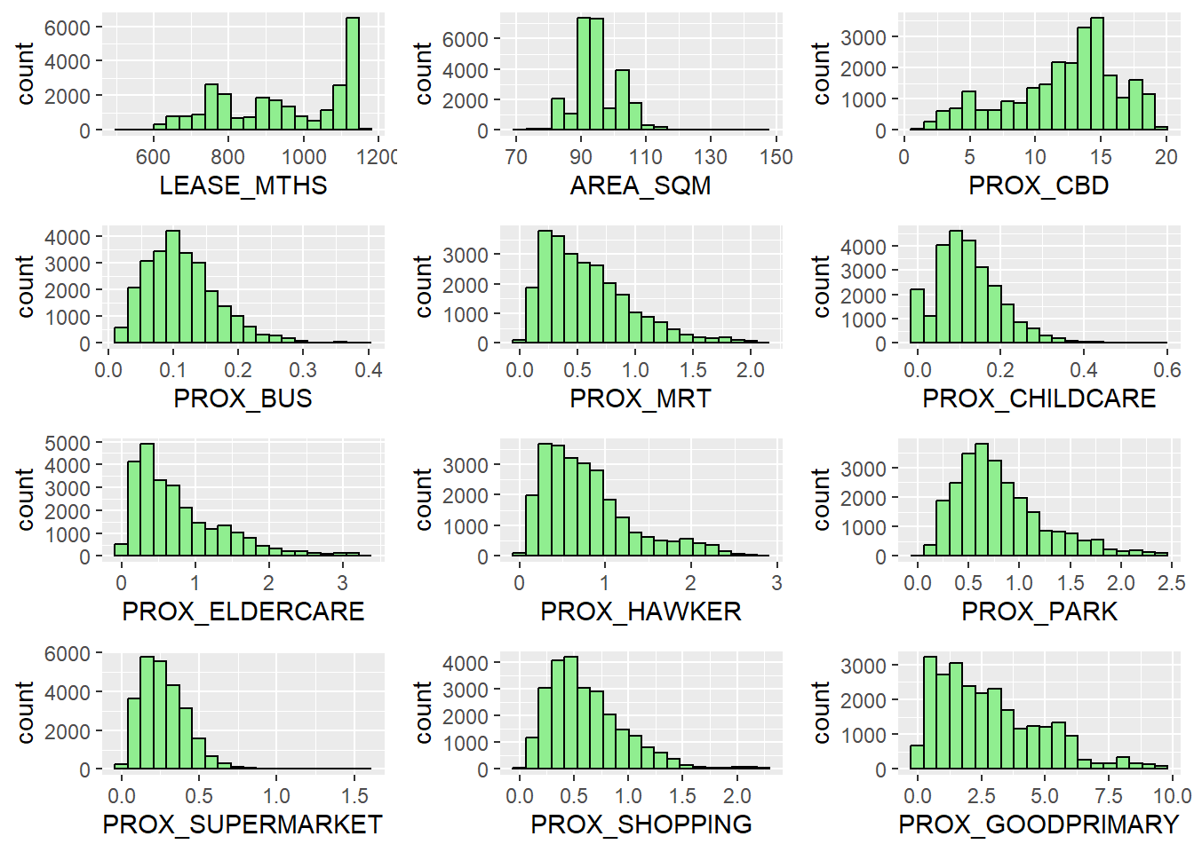
List of locational factors can be found here. Computing locational factors so it can be used to build the pricing model which will be used in the later section.

hdb_resale_main_sf <- proximity_calculation(hdb_resale_main_sf, childcare_sf, "PROX_CHILDCARE")
hdb_resale_main_sf <- proximity_calculation(hdb_resale_main_sf, elderly_care_sf, "PROX_ELDERCARE")
hdb_resale_main_sf <- proximity_calculation(hdb_resale_main_sf, hawker_centre_sf, "PROX_HAWKER")
hdb_resale_main_sf <- proximity_calculation(hdb_resale_main_sf, good_primary_school_sf, "PROX_GOODPRIMARY")
hdb_resale_main_sf <- proximity_calculation(hdb_resale_main_sf, parks_sf, "PROX_PARK")
hdb_resale_main_sf <- proximity_calculation(hdb_resale_main_sf, supermarket_sf, "PROX_SUPERMARKET")
hdb_resale_main_sf <- proximity_calculation(hdb_resale_main_sf, shopping_mall_sf, "PROX_SHOPPING")
hdb_resale_main_sf <- proximity_calculation(hdb_resale_main_sf, mrt_sf, "PROX_MRT")
hdb_resale_main_sf <- proximity_calculation(hdb_resale_main_sf, cbd_sf, "PROX_CBD")
hdb_resale_main_sf <- proximity_calculation(hdb_resale_main_sf, bus_stop_sf, "PROX_BUS")

5.4 Calculation for Location Factors with Radius

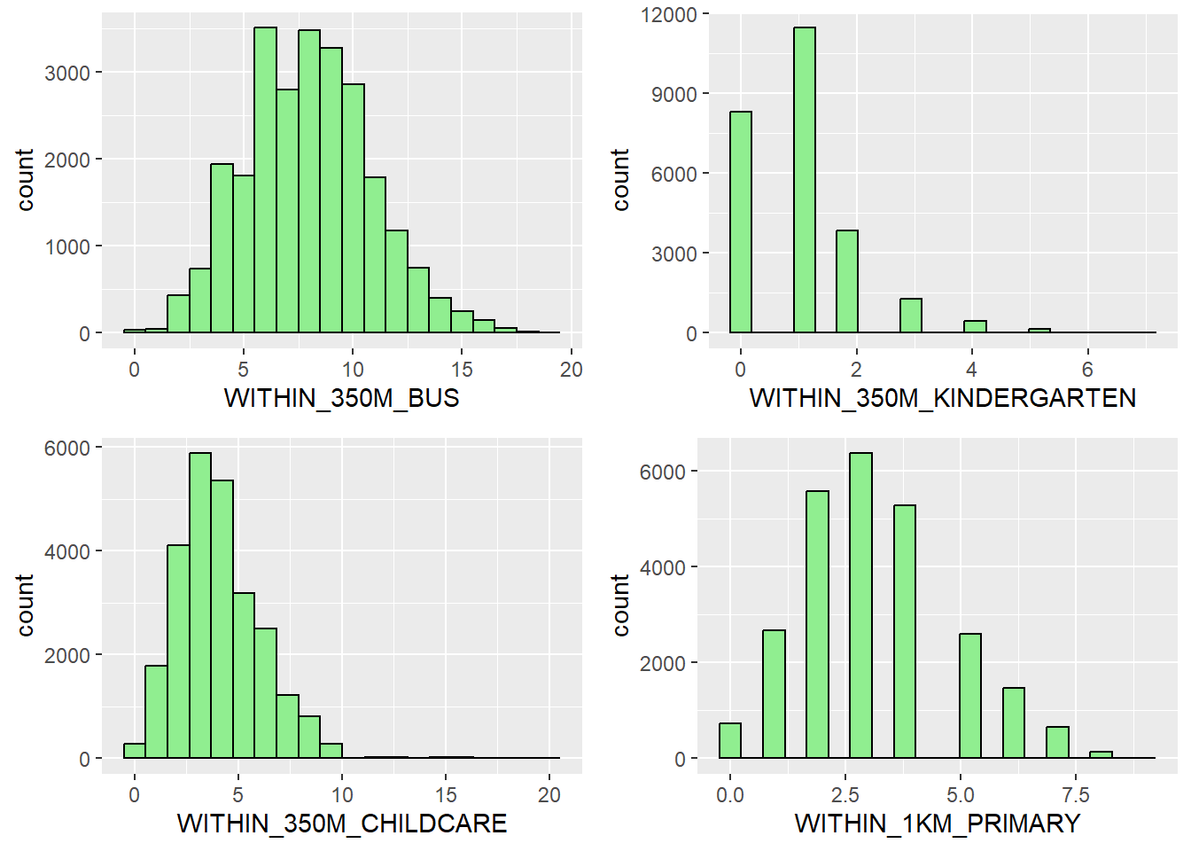
List of locational factors with radius can be found here. Computing locational factors with radius so it can be used to build the pricing model which will be used in the later section.

hdb_resale_main_sf <- proximity_radius_calculation(hdb_resale_main_sf, bus_stop_sf, "WITHIN_350M_BUS", 350)
hdb_resale_main_sf <- proximity_radius_calculation(hdb_resale_main_sf, primary_school_sf, "WITHIN_1KM_PRIMARY", 1000)
hdb_resale_main_sf <- proximity_radius_calculation(hdb_resale_main_sf, childcare_sf, "WITHIN_350M_CHILDCARE", 350)
hdb_resale_main_sf <- proximity_radius_calculation(hdb_resale_main_sf, kindergarten_sf, "WITHIN_350M_KINDERGARTEN", 350)

5.5 Saving into RDS format

Saving the hdb_resale_main_sf which consists of the proximity computation into rds format for efficient processing in the subsequent section. But before exporting it into rds format, let us rename the columns so that it is easier to interpret.

hdb_resale_main_sf <- hdb_resale_main_sf %>%
  mutate() %>%
  rename("AREA_SQM" = "floor_area_sqm",
         "PRICE" = "resale_price",
         "STOREY" = "storey_range",
         "LEASE_MTHS" = "remaining_lease_mths"
         )

Saving it into RDS format

write_rds(hdb_resale_main_sf, "data/model/hdb_resale_main.rds")

6 Exploratory Data Analysis (EDA)

6.1 Reading RDS file of HDB (that contains the proximity values

hdb_resale_main_prox_sf <- read_rds("data/model/hdb_resale_main.rds")

6.2 EDA with Statistical Graphics

6.2.1 Histogram Plot of 4 Room Resale Price

We can plot the distribution of resale price by using appropriate Exploratory Data Analysis (EDA) as shown in the code chunk below.

ggplot(data = hdb_resale_main_prox_sf, aes(x = `PRICE`)) +
  geom_histogram(bins = 20, color = "black", fill = "light green") +
  labs(title = "Distribution of 4-Room Resale Prices",
       x = "Resale Prices",
       y = "Count")

The figure above reveals a slightly right skewed distribution. This means that more 4-Room Resale prices were transacted at relatively lower prices.

6.2.2 Multiple Histogram Plots of locational factors

We can also see the distribution of the following locational factors.

LEASE_MTHS <- ggplot(data = hdb_resale_main_prox_sf, aes(x = `LEASE_MTHS`)) +
  geom_histogram(bins = 20, color = "black", fill = "light green")

AREA_SQM <- ggplot(data = hdb_resale_main_prox_sf, aes(x = `AREA_SQM`)) +
  geom_histogram(bins = 20, color = "black", fill = "light green")

PROX_CBD <- ggplot(data = hdb_resale_main_prox_sf, aes(x = `PROX_CBD`)) +
  geom_histogram(bins = 20, color = "black", fill = "light green")

PROX_BUS <- ggplot(data = hdb_resale_main_prox_sf, aes(x = `PROX_BUS`)) +
  geom_histogram(bins = 20, color = "black", fill = "light green")

PROX_MRT <- ggplot(data = hdb_resale_main_prox_sf, aes(x = `PROX_MRT`)) +
  geom_histogram(bins = 20, color = "black", fill = "light green")

PROX_GOODPRIMARY <- ggplot(data = hdb_resale_main_prox_sf, aes(x = `PROX_GOODPRIMARY`)) + geom_histogram(bins = 20, color = "black", fill = "light green")

PROX_CHILDCARE <- ggplot(data = hdb_resale_main_prox_sf, aes(x = `PROX_CHILDCARE`)) +
  geom_histogram(bins = 20, color = "black", fill = "light green")

PROX_ELDERCARE <- ggplot(data = hdb_resale_main_prox_sf, aes(x = `PROX_ELDERCARE`)) +
  geom_histogram(bins = 20, color = "black", fill = "light green")

PROX_HAWKER <- ggplot(data = hdb_resale_main_prox_sf, aes(x = `PROX_HAWKER`)) +
  geom_histogram(bins = 20, color = "black", fill = "light green")

PROX_PARK <- ggplot(data = hdb_resale_main_prox_sf, aes(x = `PROX_PARK`)) +
  geom_histogram(bins = 20, color = "black", fill = "light green")

PROX_SHOPPING <- ggplot(data = hdb_resale_main_prox_sf, aes(x = `PROX_SHOPPING`)) +
  geom_histogram(bins = 20, color = "black", fill = "light green")

PROX_SUPERMARKET <- ggplot(data = hdb_resale_main_prox_sf, aes(x = `PROX_SUPERMARKET`)) + geom_histogram(bins = 20, color = "black", fill = "light green")


ggarrange(LEASE_MTHS, AREA_SQM, PROX_CBD, PROX_BUS, PROX_MRT, PROX_CHILDCARE, PROX_ELDERCARE, PROX_HAWKER, PROX_PARK, PROX_SUPERMARKET, PROX_SHOPPING,PROX_GOODPRIMARY, ncol = 3, nrow = 4)

6.2.3 Multiple Histogram Plots of location factors with radius

WITHIN_350M_BUS <- ggplot(data = hdb_resale_main_prox_sf, aes(x = `WITHIN_350M_BUS`)) +
  geom_histogram(bins = 20, color = "black", fill = "light green")

WITHIN_350M_KINDERGARTEN <- ggplot(data = hdb_resale_main_prox_sf, aes(x = `WITHIN_350M_KINDERGARTEN`)) +
  geom_histogram(bins = 20, color = "black", fill = "light green")

WITHIN_350M_CHILDCARE <- ggplot(data = hdb_resale_main_prox_sf, aes(x = `WITHIN_350M_CHILDCARE`)) +
  geom_histogram(bins = 20, color = "black", fill = "light green")

WITHIN_1KM_PRIMARY <- ggplot(data = hdb_resale_main_prox_sf, aes(x = `WITHIN_1KM_PRIMARY`)) +
  geom_histogram(bins = 20, color = "black", fill = "light green")

ggarrange(WITHIN_350M_BUS, WITHIN_350M_KINDERGARTEN,WITHIN_350M_CHILDCARE, WITHIN_1KM_PRIMARY, ncol = 2, nrow = 2)

6.2.3 Drawing Statistical Point Map

Revealing the geospatial distribution HDB 4 room resale prices in Singapore. The map will be prepared by using tmap package.

The code chunk below is used to turn on the interactive mode of tmap.

tmap_mode("view")
tmap mode set to interactive viewing

Next, the code chunks below is used to create an interactive point symbol map.

tmap_options(check.and.fix = TRUE)
tm_shape(hdb_resale_main_prox_sf)+
  tm_dots(col = "PRICE",
          alpha = 0.6,
          style = "quantile",
             popup.vars=c("block"="block", "street_name"="street_name", "flat_model" = "flat_model", "town" = "town", "PRICE" = "PRICE", "LEASE_MTHS", "LEASE_MTHS")) +
  tm_view(set.zoom.limits = c(11, 14))

From the point map above, we can observe that the more pricey HDB 4 room resale is located in the regions of central and sourthern parts of Singapore as the points are darker in colour as compared to the western side of Singapore.

7 Regression

7.1 Visualising the relationships of the independent variables

Before building a multiple linear regression model, it is important to ensure that the indepdent variables used are not highly correlated to each other. If these highly correlated independent variables are used in building a regression model by mistake, the quality of the model will be compromised. This phenomenon is known as multicollinearity in statistics. The code chunk below is used to plot a scatterplot matrix of the relationship.

hdb_resale_main_nogeo <- hdb_resale_main_prox_sf %>%
  st_drop_geometry() %>%
  dplyr::select(c(7, 8, 11, 12, 14:27)) %>%
  mutate(STOREY = as.character(STOREY))

Plotting the Scatterplot matrix

corrplot(cor(hdb_resale_main_nogeo[, 2:18]), 
         diag = FALSE, 
         order = "AOE",
         t1.pos = "td",
         t1.cex = 0.4,
         tl.cex = 0.5,
         cl.cex = 0.6,
         number.cex = 0.6,
         method = "number",
         type = "upper")

From the above output, we can see that PROX_CBD is highly correlated with “good primary school” and “price” but the value seems to be in the acceptable range, thus we do not need to exclude this variable in the subsequent model building.

7.2 Calibrating Multiple Linear Regression Model using OLSRR

7.2.1 Training Data and Test Data

Training Data - May 2022 to December 2022 (Time period is reduced because of computation time)

hdbdata <- read_rds("data/model/hdb_resale_main.rds")

train_data <- filter(hdbdata) %>%
  filter(month >= "2022-05" & month <= "2022-12")

Test data

test_data <- filter(hdbdata) %>%
  filter(month >= "2023-01" & month <= "2023-02")

Writing training and test data to rds

write_rds(train_data, "data/model/train_data.rds")
write_rds(test_data, "data/model/test_data.rds")

Calibrating MLR model

hdb_resale.mlr <- lm(formula = PRICE ~ STOREY + AREA_SQM + PROX_BUS + PROX_CBD +
                    PROX_CHILDCARE + PROX_ELDERCARE + PROX_GOODPRIMARY +
                   PROX_HAWKER + PROX_MRT + PROX_PARK + PROX_SHOPPING +
                   PROX_SUPERMARKET + WITHIN_1KM_PRIMARY + WITHIN_350M_BUS +
                   WITHIN_350M_CHILDCARE + WITHIN_350M_KINDERGARTEN + LEASE_MTHS,
                 data = train_data)

Summary of MLR Model

summary(hdb_resale.mlr)

Call:
lm(formula = PRICE ~ STOREY + AREA_SQM + PROX_BUS + PROX_CBD + 
    PROX_CHILDCARE + PROX_ELDERCARE + PROX_GOODPRIMARY + PROX_HAWKER + 
    PROX_MRT + PROX_PARK + PROX_SHOPPING + PROX_SUPERMARKET + 
    WITHIN_1KM_PRIMARY + WITHIN_350M_BUS + WITHIN_350M_CHILDCARE + 
    WITHIN_350M_KINDERGARTEN + LEASE_MTHS, data = train_data)

Residuals:
    Min      1Q  Median      3Q     Max 
-200506  -40057    -196   35953  341505 

Coefficients:
                           Estimate Std. Error t value Pr(>|t|)    
(Intercept)              117465.972  13138.303   8.941  < 2e-16 ***
STOREY04 TO 06            20880.768   2228.092   9.372  < 2e-16 ***
STOREY07 TO 09            34078.539   2250.294  15.144  < 2e-16 ***
STOREY10 TO 12            43053.605   2311.823  18.623  < 2e-16 ***
STOREY13 TO 15            46633.301   2752.214  16.944  < 2e-16 ***
STOREY16 TO 18            62972.858   3630.415  17.346  < 2e-16 ***
STOREY19 TO 21            84808.627   5149.465  16.469  < 2e-16 ***
STOREY22 TO 24            97224.707   6167.681  15.764  < 2e-16 ***
STOREY25 TO 27           149654.452   6562.323  22.805  < 2e-16 ***
STOREY28 TO 30           187209.624   7242.305  25.849  < 2e-16 ***
STOREY31 TO 33           198013.496  10124.077  19.559  < 2e-16 ***
STOREY34 TO 36           210554.575   9003.768  23.385  < 2e-16 ***
STOREY37 TO 39           237699.829  10876.248  21.855  < 2e-16 ***
STOREY40 TO 42           227252.466  18837.716  12.064  < 2e-16 ***
STOREY43 TO 45           360037.438  22477.170  16.018  < 2e-16 ***
STOREY46 TO 48           612383.921  58985.198  10.382  < 2e-16 ***
STOREY49 TO 51           503783.066  41787.013  12.056  < 2e-16 ***
AREA_SQM                   3518.664    106.303  33.100  < 2e-16 ***
PROX_BUS                  38235.816  13449.431   2.843  0.00448 ** 
PROX_CBD                 -16708.867    242.987 -68.765  < 2e-16 ***
PROX_CHILDCARE           -20276.935   9280.430  -2.185  0.02893 *  
PROX_ELDERCARE            -7653.325   1210.921  -6.320 2.76e-10 ***
PROX_GOODPRIMARY          -3163.448    439.746  -7.194 6.91e-13 ***
PROX_HAWKER              -21991.871   1458.533 -15.078  < 2e-16 ***
PROX_MRT                 -26467.485   1993.721 -13.275  < 2e-16 ***
PROX_PARK                 -2425.358   1581.844  -1.533  0.12526    
PROX_SHOPPING            -23289.525   2337.896  -9.962  < 2e-16 ***
PROX_SUPERMARKET          14418.693   4617.801   3.122  0.00180 ** 
WITHIN_1KM_PRIMARY        -9733.878    545.347 -17.849  < 2e-16 ***
WITHIN_350M_BUS            1230.797    266.079   4.626 3.80e-06 ***
WITHIN_350M_CHILDCARE     -3461.504    400.097  -8.652  < 2e-16 ***
WITHIN_350M_KINDERGARTEN   6418.913    758.569   8.462  < 2e-16 ***
LEASE_MTHS                  386.242      4.847  79.682  < 2e-16 ***
---
Signif. codes:  0 '***' 0.001 '**' 0.01 '*' 0.05 '.' 0.1 ' ' 1

Residual standard error: 58860 on 7497 degrees of freedom
Multiple R-squared:  0.7955,    Adjusted R-squared:  0.7946 
F-statistic: 911.1 on 32 and 7497 DF,  p-value: < 2.2e-16

Reading and Writing to rds

write_rds(hdb_resale.mlr, "data/model/hdb_resale.mlr.rds")
hdb_resale.mlr <- read_rds("data/model/hdb_resale.mlr.rds")

7.2.1 Predict MLR Model

mlr_pred <- predict(hdb_resale.mlr, test_data)

write_rds(mlr_pred, "data/model/mlr.pred.rds")

Converting predicting output into a dataframe

mlr_pred_df <- as.data.frame(mlr_pred)

7.2.2 Calculate RMSE

In the code chunk below, cbind() is used to append the predicted values onto test_data_p_mlr

test_data_p_mlr <- cbind(test_data, mlr_pred)

The root mean square error (RMSE) allows us to measure how far predicted values are from observed values in a regression analysis. In the code chunk below, rmse() of Metrics package is used to compute the RMS

rmse(test_data_p_mlr$PRICE, 
     test_data_p_mlr$mlr_pred)
[1] 62709.34

The above output shows the RMSE value is 62709.34.

7.3 Test for Non-linearity

In multiple linear regression, it is important for us to test the assumption that linearity and additivity of the relationship between dependent and independent variables.

In the code chunk below, the ols_plot_resid_fit() of olsrr package is used to perform linearity assumption test.

ols_plot_resid_fit(hdb_resale.mlr)

The figure above reveals that most of the data points are scattered around the 0 line, hence we can safely conclude that the relationships between the dependent variable and independent variables are linear.

7.4 Test for Normality Assumption

Lastly, the code chunk below uses ols_plot_resid_hist() of olsrr package to perform normality assumption test.

ols_plot_resid_hist(hdb_resale.mlr)

The figure reveals that the residual of the multiple linear regression model (i.e. hdb_resale.mlr) is resemble normal distribution.

7.5 Predictive Model for Geographic Random Forest

Loading rds file to get training and test data

hdbdata <- read_rds("data/model/hdb_resale_main.rds")

7.6 Preparing Coordinates Data

7.6.1 Extracting coordinates data

coords <- st_coordinates(hdbdata)
coords_train <- st_coordinates(train_data)
coords_test <- st_coordinates(test_data)

7.6.2 Saving and Reading into RDS

coords <- write_rds(coords, "data/model/coords.rds")
coords_train <- write_rds(coords_train, "data/model/coords_train.rds" )
coords_test <- write_rds(coords_test, "data/model/coords_test.rds" )

Read RDS

coords<-read_rds("data/model/coords.rds")
coords_train<-read_rds("data/model/coords_train.rds")
coords_test<-read_rds("data/model/coords_test.rds")

7.6.3 Dropping Geometry fields

train_data_nogeo <- train_data %>%
  st_drop_geometry()

7.7 Calibrating Geographical Random Forest Model

7.7.1 Computing bandwidth

Setting seed to make the code reproducible and setting trees to 30 to reduce computation time.

set.seed(1234)
gwRF_bw <- grf.bw(formula = PRICE ~ STOREY + AREA_SQM + PROX_BUS + PROX_CBD +
                   PROX_CHILDCARE + PROX_ELDERCARE + PROX_GOODPRIMARY +
                   PROX_HAWKER + PROX_MRT + PROX_PARK + PROX_SHOPPING +
                   PROX_SUPERMARKET + WITHIN_1KM_PRIMARY + WITHIN_350M_BUS +
                   WITHIN_350M_CHILDCARE + WITHIN_350M_KINDERGARTEN + 
                  LEASE_MTHS, 
                  train_data_nogeo, kernel = "adaptive", coords = coords_train, trees=30)

It the span of 28 hours, only 366 bandwidths were generating :( and the code chunk has not ran finished. Due to the lack of time, i picked the highest R2 value and took is bandwidth value to be used to generate the model. The image below represents the bandwidth with the highest r2 value.

#setting bandwidth value and assign it to variable
adaptive_bw_grf<-477

7.7.2 Constructing Model

set.seed(1234)
gwRF_adaptive<-grf(formula = PRICE ~ STOREY + AREA_SQM + PROX_BUS + PROX_CBD +
                   PROX_CHILDCARE + PROX_ELDERCARE + PROX_GOODPRIMARY +
                   PROX_HAWKER + PROX_MRT + PROX_PARK + PROX_SHOPPING +
                   PROX_SUPERMARKET + WITHIN_1KM_PRIMARY + WITHIN_350M_BUS +
                   WITHIN_350M_CHILDCARE + WITHIN_350M_KINDERGARTEN + 
                  LEASE_MTHS, 
                   dframe=train_data_nogeo,
                   bw=adaptive_bw_grf,
                   kernel="adaptive",
                   coords=coords_train,
                   ntree=50)

# saving the result as an rds 
write_rds(gwRF_adaptive, "data/model/gwRF_adaptive.rds")

7.7.3 Prediction

7.7.3.1 Preparing Test Data

Combining the test data with the corresponding coordinates data.

test_data_pred <- cbind(test_data, coords_test) %>%
  st_drop_geometry()

write_rds(test_data, "data/model/test_data_pred.rds")

7.7.3.2 Predicting with Test Data

gwRF_adaptive<-read_rds("data/model/gwRF.rds")

gwRF_pred <- predict.grf(gwRF_adaptive, 
                           test_data_pred, 
                           x.var.name="X",
                           y.var.name="Y", 
                           local.w=1,
                           global.w=0)

GRF_pred <- write_rds(gwRF_pred, "data/model/GRF_pred.rds")

7.7.3.3 Converting output to data frame

The output of the predict.grf() is a vector of predicted values. It is wiser to convert it into a data frame for further visualisation and analysis.

GRF_pred <- read_rds("data/model/GRF_pred.rds")
GRF_pred_df <- as.data.frame(GRF_pred)

In the code chunk below, cbind() is used to append the predicted values onto test_data

test_data_p <- cbind(test_data, GRF_pred_df)

7.7.4.4 Calculating RMSE

The root mean square error (RMSE) allows us to measure how far predicted values are from observed values in a regression analysis. In the code chunk below, rmse() of Metrics package is used to compute the RMSE.

rmse(test_data_p$PRICE, 
     test_data_p$GRF_pred)
[1] 56525.02

8 Conclusion

rmse(test_data_p_mlr$PRICE, 
     test_data_p_mlr$mlr_pred)
[1] 62709.34

Alternatively, scatterplot can be used to visualise the actual resale price and the predicted resale price by using the code chunk below.

ggplot(data = test_data_p_mlr,
       aes(x = mlr_pred,
           y = PRICE)) +
  geom_point()

rmse(test_data_p$PRICE, 
     test_data_p$GRF_pred)
[1] 56525.02

Alternatively, scatterplot can be used to visualise the actual resale price and the predicted resale price by using the code chunk below.

ggplot(data = test_data_p,
       aes(x = GRF_pred,
           y = PRICE)) +
  geom_point()

Analysis

RMSE Definition: The Root Mean Squared Error (RMSE) is one of the two main performance indicators for a regression model. It measures the average difference between values predicted by a model and the actual values. It provides an estimation of how well the model is able to predict the target value (accuracy).

From the above table comparison between OLS (Ordinary Least Square) and GRF (Geographical Random Forest), we can see that GRF is better used to predict the resale prices of the 4 room as the RMSE value (56.525.02) was lesser.

There are some limitations to this assignment as well. Supposedly the number of trees used in building the model was supposed to be higher but due to hardware limitations, lesser trees was used. This could suggest a potentially better model.

9 Miscellaneous

9.1 Calibrating GRF Model with 70 Trees

The below code chunks will be similar to Section 7.7 onwards. Just that 70 Trees will be used to build the model.

set.seed(1234)
gwRF_adaptive_extra<-grf(formula = PRICE ~ STOREY + AREA_SQM + PROX_BUS + PROX_CBD +
                   PROX_CHILDCARE + PROX_ELDERCARE + PROX_GOODPRIMARY +
                   PROX_HAWKER + PROX_MRT + PROX_PARK + PROX_SHOPPING +
                   PROX_SUPERMARKET + WITHIN_1KM_PRIMARY + WITHIN_350M_BUS +
                   WITHIN_350M_CHILDCARE + WITHIN_350M_KINDERGARTEN + 
                  LEASE_MTHS, 
                   dframe=train_data_nogeo,
                   bw=adaptive_bw_grf,
                   kernel="adaptive",
                   coords=coords_train,
                   ntree=70)

# saving the result as an rds object
write_rds(gwRF_adaptive_extra, "data/model/gwRF_adaptive-extra.rds")

Predicting with test data

gwRF_pred_extra <- predict.grf(gwRF_adaptive_extra, 
                           test_data_pred, 
                           x.var.name="X",
                           y.var.name="Y", 
                           local.w=1,
                           global.w=0)

GRF_pred_extra <- write_rds(gwRF_pred_extra, "data/model/GRF_pred_extra.rds")

Reading the Prediction file generated and converting output to data frame

GRF_pred_extra <- read_rds("data/model/GRF_pred_extra.rds")
GRF_pred_df_extra <- as.data.frame(GRF_pred_extra)

cbind() is used to append the predicted values onto test_data

test_data_p_extra <- cbind(test_data, GRF_pred_df_extra)

Calculating RMSE

rmse(test_data_p_extra$PRICE, 
     test_data_p_extra$GRF_pred)
[1] 56685.62
Analysis

Making a comparison of the earlier GRF model building which uses 50 trees, the RMSE value was 56525.02. However when the GRF model was build with 70 trees, the RMSE value increased to 56685.62. This shows that not necessarily increasing the number of trees will result in a better model.

Comparing RMSE value (56685.62) which uses 70 trees to build the model to RMSE value (56525.02) which uses 50 trees to build the model, this shows that not necessarily setting higher trees to build the model would result in a better model.

10 References

Credits to Prof Kam’s In Class Exercises, Senior Megan’s Work and classmates who helped in the data gathering.