In-Class Exercise 6

Getting Started

Installing and Loading the R Packages

Three R packages will be used need for this in-class exercise, they are: sf, sfdep and tidyverse.

Do it Yourself!

Using the steps you learned in previous lesson, install and load sf, tmap, sfdep and tidyverse packages into R environment

pacman::p_load(sf, tmap, sfdep, tidyverse)

The Data

For the purpose of this in-class exericse, the Human data sets will be used.

There are two data sets in this use case, they are:

• Hunan, a geospatial data set in ESRI shapefile format, and

• Hunan_2021, an attribute data set in csv format.

Importing geospatial data

Do it Yourself!

hunan <- st_read(dsn ="data/geospatial", 
                 layer = "Hunan")

Reading layer `Hunan' from data source 
  `C:\HoYongQuan\IS415-GAA(New)\In-Class_Ex\In-Class_Ex06\data\geospatial' 
  using driver `ESRI Shapefile'
Simple feature collection with 88 features and 7 fields
Geometry type: POLYGON
Dimension:     XY
Bounding box:  xmin: 108.7831 ymin: 24.6342 xmax: 114.2544 ymax: 30.12812
Geodetic CRS:  WGS 84

#contiguity can use this dataset, because of geographic coordinate system.

Importing attribute table

hunan2012 <- read_csv("data/aspatial/Hunan_2012.csv")

#didnt load readr in pacman, because this package is part of tidyverse

Combining both data frame by using left join

Important

In order to retain the geospatial properties, the left data frame must be the sf data.frame (i.e. hunan)

hunan_GDPPC <- left_join(hunan, hunan2012)%>%
  select(1:4, 7, 15)
#retain column 1 to 4, 7 and 15

Plotting a choropleth map

tmap_mode("plot")
tm_shape(hunan_GDPPC) +
  tm_fill("GDPPC",
          style = "quantile",
          palette = "Blues",
          title = "GDPPC") +
  tm_layout(main.title = "Distribution of GDP per capita by district, Hunan Province",
            main.title.position = "center",
            main.title.size = 1.2,
            legend.height = 0.45,
            legend.width = 0.35,
            frame = TRUE) +
  tm_borders(alpha = 0.5) +
  tm_compass(type="8star", size = 2) + 
  tm_scale_bar() +
  tm_grid(alpha = 0.2)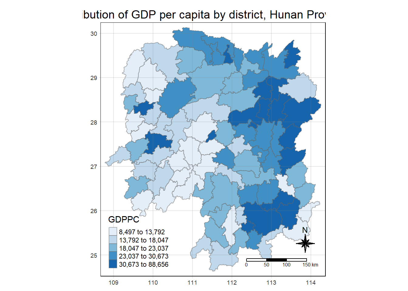

#Classification: Regional Economics, Equal interval range

Deriving Contiguity Spatial Weights

Contiguity neighbours method: Queen’s method

In the code chunk below, st_contiguity() is used to derive a contiguity neighbour list by using Queen’s method.

cn_queen <- hunan_GDPPC %>%
  mutate(nb = st_contiguity(geometry),
         .before = 1)

#mutate - create new field
#.before = 1 = put newly created field at the first column
#nb format c(2,3,4,57,85), numbers in the bracket represents the row name

The code chunk below is used to print the summary of the first lag neighbour list (i.e. nb)

#summary(nb_queen$nb)

Do it Yourself!

Using the steps you just learned, derive a contiguity neighbour list using Rook’s method

cn_rook <- hunan_GDPPC %>%
  mutate(nb= st_contiguity(geometry),
         queen = FALSE,
         .before = 1)

Computing Contiguity weights

Contiguity weights: Queen’s method

wm_q <- hunan_GDPPC %>%
  mutate(nb = st_contiguity(geometry),
         wt = st_weights(nb),
         .before = 1)

#nb is list

Contiguity weights: Rook’s method

wm_r <- hunan %>%
  mutate(nb = st_contiguity(geometry),
         queen = FALSE,
         wt = st_weights(nb),
         .before = 1)